LIS 572 Oregon Logs Data Project

LIS 572: Data Science with Professor Melanie Walsh.
By William Wu and Ben Hauptman.
First published: 2022-12-04.
Updated with weighted values: 2022-12-05.

Introduction

The question we looked into was if macroeconomic swings could be detected through the price of logs. We used a dataset provided by the Oregon Department of Forestry. We chose this dataset because Oregon is a large supplier of logs throughout the Northwest.

(Note, Pond Value refers to the price paid for an unprocessed log at a processing plant. Where the logs are stacked are called “Ponds”. Log price and pond value are the same).

Since we knew that Douglas Fir is very common in Oregon, and since we also knew that Douglas Fir is comomnly used in building construction, we predicted that data analysis on this dataset would indeed produce results that clearly show the economic crisis of 2008.

The dataset can be found here: Oregon Log Prices Dataset.
Our code can be found here: Oregon Log Prices R Analysis.

Context Concerning the Dataset from the Oregon Department of Forestry

The dataset that we decided to use was from the Oregon Department of Forestry. The raw dataset has 7,884 distinct rows of data about sold logs over the course of 15 years, from 2000 to 2015. It also contains some data from 2016, but because the data is incomplete for that year we decided against using it as part of our analysis and final dataset. (We will talk more about our computational process below). The raw dataset has seven different variables tracked for each column, with those variables being:

1. The Year it was sold
2. The Quarter it was sold in that year
3. what Region the log came from
4. The Species of log
5. The Grade it was given
6. The price it was sold for (“Pond Value”), and
7. The number of people who bid on the log / the number of pond centers called. (“Quote”).

Ethical Concerns

There does not seem to be any glaring ethical concerns, mostly because none of the pond processing plants are identified by name, nor are any specific geo-located logging coordinates expressed anywhere in the dataset or on the government website.

Apart from the dataset itself, there may be environmental ethical concerns over logging, and whether or not this dataset and our analysis may encourage further exploitation and destruction of Oregon’s forests, which is depleting at an alarming rate.

Some Issues with Column Variables

The main issue with the data is that we have been unable to get in contact with the data collector/creator/curator (Julie from the Oregon Department of Forestry). Without her help, we are unable to use one of the column variables at all (Grade), and we are not 100% certain of the meaning of one of two of the column variables (Quotes, Year).

First, let it be known that Grade refers to both the size/shape and quality/purpose of the logs. As you can probably tell, with four sub-variables exsisting in one column variable, it becomes very difficult to make any interpretations, especially when they are often intermingled. For example, some rows were labled just 2P (quality and use of wood), others were labled just 8”-14” (size), and some were labled with both 3S (12”+). We think that there is likely some overlap in grading, which means that we cannot effectively use this variable. Luckily, we did not need to use Grade in our analysis to be able to help answer our question. For those who are interested in seeing how grades as a whole is calculated in Oregon, here is a quick government guide.

Second, we are unsure of what the column variable Number of Quotes means exactly. It could be the number of quotes taken per quarter fat that listed price from different processing centers, or it could be the number of logs sold at that price quoted from various pond centers. Without this exact information, we would not know if quotes would indicate a weighting system. If the former, then each row would be weighted as 1. If the latter, then each row would be weighted according to the number of quotes listed. Also, even if the value did indicate weight, we would not know by how much, because a quote from any pond center could indicate any number of logs. This is because unique pond centers are not listed as a column variable. Ultimatley, we decided to use the Quotes values as weights in themselves. Because not using quotes produces a drastically undervalued dataframe, using them should produce something closer to reality. However, it still highly likely the case that total prices in our graphs are greatly under the reality.

A final problem was the issue of Year. Does Year mean fiscal year? Or is it simply just calendar year? This problem did not really impact most of the dataset, except for the crucial years around 2007-2009. If Year means Fiscal Year, then Pond Values would not be predictive of the Great Recession. If Year means calendar year, then it could be argued that pond values may have the power to predict housing market crashes! This is because the meaning of Year would change the position of Quarter 4, which could be either seen as a predictive element or a lagging element in relation to the Great Recession. (US fiscal year starts with Quarter 1 in October).
Given the absence of information, we have taken Year to mean Fiscal Year, as Quarter (1, 2, 3, 4) is usually used in a fiscal sense. This assumption seems to correlate with exsisting government information on home sales’ prices. (Sales prices of new homes in the US).

Computational Method and Analysis

The raw dataset contains 7,884 distinct rows of information. Although already in quite good shape, we decided to further clean the data for a few reasons.

The very first thing we did was to remove three rows with N/A for prices. Pond value is the most important variable in our study, so rows without them were removed.

Next, we noticed that the data collection for 2016 was incomplete: that final year was missing quarters 3 and 4. Doing a quick group_by and count, we were able to see the distribution of the number of rows per year. As expected, 2016 had an abnormally low number of rows. We therefore completley deleted any rows which contained the year 2016. This left us with a remainder of 7,623 rows of information.

Dataset rows per year

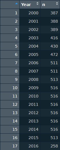
One other issue we noticed was that the number of rows was slowly ramping up from 2000-2006, and then stabailized after 2007. Is the ramping up indicitive of a larger macro logging industry trend, or is it reflective of the building up of logging industry contacts as this dataset first started (and therefore indicating a lack of information in the first years of data collection)? Without a response from Julie, we do not know.

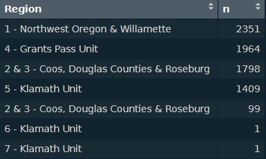
On a more specific level, while doing analysis on regions, we noticed that two regions only had a frequency of 1. These two rows were “6 - Klamath Unit” and “7 - Klamath Unit”. However, Klamath Unit already exsists as region 5. So we decided to slice those two out. Further along in our analysis on regions, we noticed that two regions were the exact same, but for some reason were split into two rows. We merged those two rows into one. (“2 & 3 - Coos, Douglas Counties & Roseburg”).

Region Count Raw

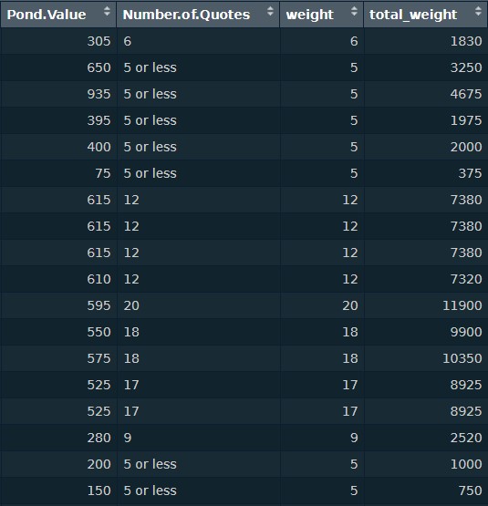
Finally, the major issue we encountered was fixing the weight problem to the best of our ability. Because the standalone prices for each row are not weighted, we had to calculate weights for them using the Quotes column. First, we used as.numeric and regmatches to strip the column of anything that was not a numeric value, which left us with only numbers. Then we added the numbers to a new column in the same dataframe, calling it ‘weight’. Finally, we multipled ‘weight’ by ‘Pond.Value’, to get the ‘total_weight’. This gave us a much more accurate picture of the total amount of prices floating around as opposed to our earlier on when we did our entire analysis based off of just single pond values.

For our analysis of the three main relationships, our most common code pattern was to group_by and then summarize(sum()) the cleaned dataset.

yearly_price_total <- 
  log_prices_clean_2 %>% 
  group_by(Year) %>% 
  summarize(Pond.Value=sum(Pond.Value))

This worked well for the relationships we were looking at:

1. Total Pond Value over Years
2. Quartlery Pond Values over Years
3. Pond Value by Species
   (Note that the Pond Value in each relationship refers to the aggregate Pond Value for each row in the targeted group_by variable).

Analysis

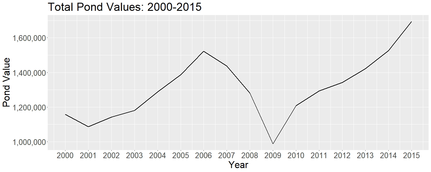
The main insight from our analysis is that economic trends have a huge impact on log prices, and this impact is reflected clearly in the data. Perhaps it can even be said that the log prices may predict economic trends, as we see pond values fall even in 2007, before the Great Recession really kicks down the door. Looking at Figure 1, we can clearly see rising pond values from 2002-2007, and the subsequent nosedive in value during the Great Recession which started in December of 2007. Pond values dropped more than 30% in the span of just 2007-2009. The price nadir of 2009 was lower than anything else we had data on.

We can also see the tail end of the drop in prices of the decade long Dotcom Bubble. Comparatively speaking, the fall in prices at the end of the Dotcom Bubble in 2000-2002 was much more gentle than the extremely steep fall in prices during the Great Recession.

Note also the great increase in prices after 2009, which reflects the massive printing of money by the Federal Reserve and the reluctance by Obama and Yellen to reduce the interest rate. Although these actions may have helped grow the economy, it has only helped to create another bubble, one which are now facing right now. Furthermore, the incredibly rapid growth and rampant printing of money has allowed get rich schemes and companies to pop up left and right, and has greatly increased uncontrolled consumerist demand among the people. For example, note all the collapsed schemes in the crypto world (FTX), or in scilicon valley (Theranos), the effects and conseqeuences of which we are just starting to see unfold in the courts todays.

Thus, despite the above mentioned problem of lacking a true weighted variable to calculate actual number of logs, we were still able to see a very clear trend. We suspect that this is because the Oregon Department of Forestry likely has a policy in place which mandates some sort of equal selection of tree grade cutting, so that no one tree growth is cut in toto.

Figure 1:

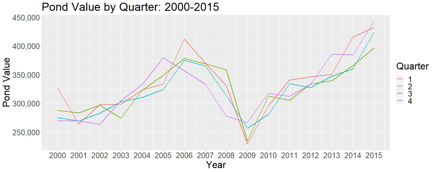
Next, in Figure 2, we can see that the quarterly values are not the most equal. Although in the past logging was highly seasonal, not only because people had nothing to do in the winter, but also because winter was when the ground was hard enough to drag logs, modern logging has become so effective that it can operate in any season. Furthermore, because of modern transportation, modern logging does not have to take place along rivers (which is why most major cities are located along big rivers: that’s where they can best accumulate wood.)

Therefore, we cannot draw any concrete conclusions from the small variations in quarterly price. Furthermore, we cannot draw conclusions because we do not have a true weight variable (as mentioned before, “Quotes” is not a true weight variable). (For more information on humanity’s interaction with trees, one should look into Deforesting the Earth by Michael Williams).

Figure 2:

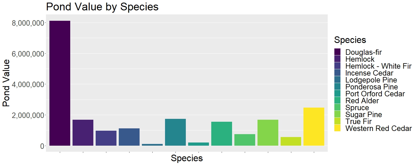
Continuing on to Figure 3, we can see why Oregon’s official state tree is the Douglas Fir. Out of the $20,953,065 grand total pond value in our calculation, the Douglas Fir holds the Douglas Fir holds 38.72% of sales! (At $8,113,795). The dataset clearly reflects the natural prevalence of the Douglas Fir in Oregon, but also displays its importance to the local rural logging economy and to the wider construction/real estate business.

Figure 3:

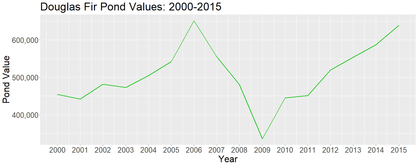
Even when we zoom into looking at the price of Douglas Fir over time we can see the same economic turns reflected.

Figure 4:

Finally, after normalizing both Total Yearly Pond Value and Total Yearly Douglas Fir Pond Value, we see that the scale of change is very similar. (The normalizing process we used was to divide each year’s price by the average of all the years).

Figure 5:

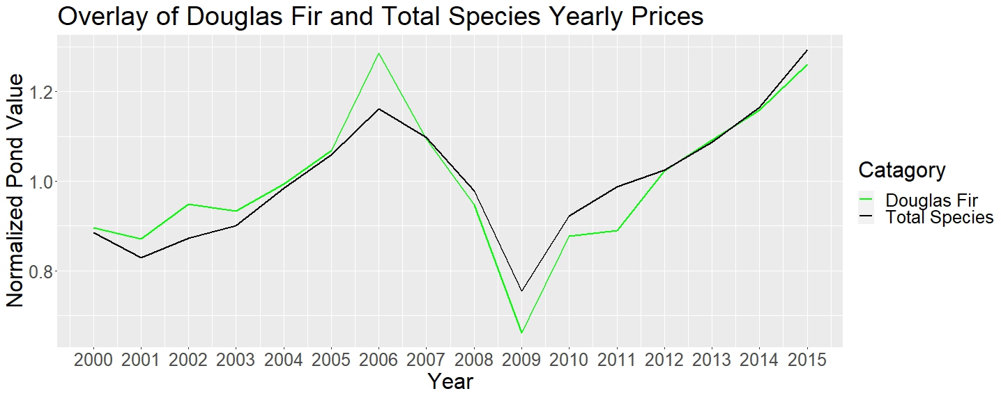
We assess that the extra increase in price of Douglas Fir at the apex of the housing bubble and the extra decrease in price at the nadir of the housing bubble are due to the fact that Douglas Fir is an indispensable and mass-logged species. Thus, during peak construction demand, you can never have enough, whereas when the housing boom ended, you will always have too much. Otherwise, the difference in the changes in price between Douglas Fir and the Aggregate Species’ Totals is not so drastic as to warrant further investigation.

Reflections

One possible direction this data could go would be to expand the current dataset to gain a much longer view of the ups and downs of log market prices. This could go both into the future and into the past, but work would have to be done to adjust prices relative to the current year’s level of inflation. It would also be interesting to compare the data against other states’ logging information, Federal logging information, and the logging information of other countries.

Finally, we just want to reiterate that the major problem we encountered was the lack of a proper weighting variable, due to the fact that we could not confirm what “Quotes” actually meant. It is highly likely “Quotes” is not truly representative as a weighting variable, due to the fact that one quote value does not indiciate how many logs are included in that one quote. However, having a number of quotes is better than no weight variable at all.

If Julie ever responds to us, it would be very interesting to see if the graphs change, depending on if we can obtain better weighting data. It is possible that we got very lucky with our current graphs, as they match our predictions and reflect historical ecnomic swings. However, in the future, it would be best to fully ascertain the meaning and weighting of all variables.